Detailed Methods: Mapping a Conservation Vision

All data sources used to map the individual components of the Cumulative Conservation Values map can be found here: Table S1. Data sources for conservation values mapping.

Ecological Values

We took a coarse-filter/fine-filter approach to manage the complex organization of biological systems and the practical limits of existing data and knowledge [40]. The practical advantage of this approach is that it makes the best use of available data to represent the full range of representative biodiversity with a reasonable number of biodiversity elements. Our knowledge regarding species ranges and habitat needs will always be incomplete; species data are limited and dependent on survey effort, and therefore, prone to vary in geographic coverage. Conversely, spatial data on coarse filter features such as ecosystem types are typically easy to access, updated semi-regularly and usually employ classification schemes that are consistent across geographies. The coarse-filter/fine-filter approach is designed to overcome the common challenges of uneven (in extent and quality) data coverage to yet create a conservation vision that credibly captures the range of ecological actors in a landscape and the intricate ways in which they organize and sort themselves.

We used the Ecological Mapping Systems of Texas [41] produced by the Texas Parks & Wildlife as the base for the coarse-filter, habitat-centric approach. We aggregated the ecological mapping systems into NatureServe habitat classes (i.e., forests & woodland savannas, grassland & herbaceous vegetation, herbaceous wetlands, shrublands, sparsely vegetated areas, woody wetlands & riparian areas) to represent the coarse-filter habitats (for full crosswalk, see Table S2. Crosswalk of the Ecological Mapping Systems of Texas and NatureServe classes). We also updated three landcover classes (riparian areas, cliffs/crevices and converted lands) on the recommendation of the science subcommittee, because the current mapping of the classes were considered incomplete. We added in surface waters as mapped by the Texas Natural Resource Information System (TNRIS)[42] for the norther portion of Presidio county where they were missing. We also added in areas with slopes greater than 24 degrees in the counties of Crockett, Terrell and Val Verde to represent cliff areas in the Devils and Pecos River watersheds. Finally, we used the National Land Cover Database 2016 Developed Imperviousness (CONUS) [43–45] to update areas converted to impervious surfaces (i.e., roads, energy development, settled areas). 

We then inventoried species (n = 516, for full list of species, see Table S3. Fine-filter species and habitat associations and Table S4. Summary of distribution of fine-filter species by taxonomic group, Texas SGCN status, global ranks, state protection status and habitat association) with economic, iconic and conservation value in the region [46–48]. We selected three wide-ranging species (pronghorn, bighorn sheep and mountain lion) for further attention and produced habitat suitability and connectivity models as part of the fine-filter focus. We describe our methods in general details below.

Intact Landscapes

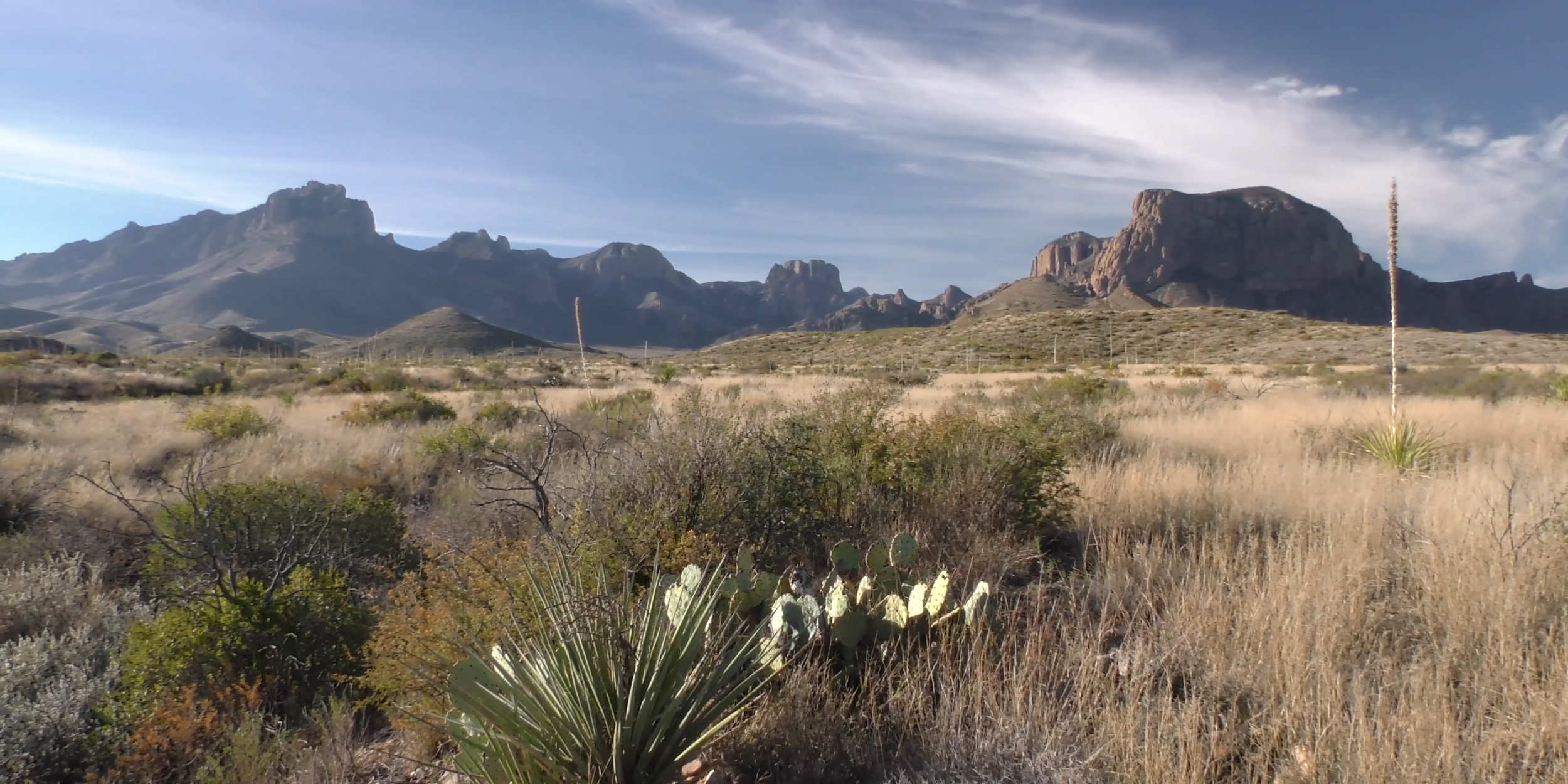
Intact landscapes represent large, unfragmented patches of different habitat types with low levels of modification from human pressures. Expanses of unfragmented natural habitat, such as grasslands and shrublands, tap into the sense of the remote and “wide-open” landscapes that stakeholders identified as a central characteristic of the region. 

Intact landscapes are ecologically important as well. Intact ecosystems are better positioned to support the long-term persistence of a full range of species who have their own individual minimum home area size requirements and needs for connected habitat. Fragmentation and habitat loss can lead to concerning population declines of iconic biodiversity residents of a place. Moreover, the habitat degradation that often follows significant fragmentation and loss can weaken an ecosystem’s ability to withstand and recover from most natural disturbances (e.g., drought, erosion, fire).

To identify instances of intact landscapes off similar landcover types, we grouped 116 vegetation types from the Ecological Mapping Systems of Texas to five broad NatureServe systems classes:

• Forests and woodland savannas

• Herbaceous vegetation/grasslands

• Herbaceous wetlands

• Chihuahuan desert shrublands

• Woody wetlands and riparian

We applied size thresholds and a measure of condition for each patch to identify the set of best examples of each system [41, 47–49]. Size thresholds aim to estimate the minimum area required for an ecosystem type to be considered functionally able to sustain itself and the biota it supports over the long term. 

We used a cumulative measure of human modification of terrestrial lands as an indirect measure of the condition of a patch. Human modification is represented as an integrated index of the physical extent and intensity of 10 anthropogenic pressures on the land. These stressors include: residential development, urban/commercial development, crop and pastureland, oil and gas wells, mines, concentrated/PV solar, wind farms, road footprint, railways and above-ground powerlines [50, 51]. Areas with multiple stressors are considered more degraded than areas with single stressors. We set ecologically-informed thresholds to delineate areas of low, moderate and high degrees of human modification [50, 51]. 

In the final step, intact landscapes are those ecosystem patches that are above a minimum moderate threshold size and are in the best condition as measured by the cumulative human modification index (Table S5). Because riparian and wetland resources were considered so essential in this arid landscape, we swept in all patches regardless of size, although we prioritized those in good condition over those which scored a heavily impacted by human activities per the human modification index. 

Grasslands & Riparian & Wetland Areas, Springs

The Stakeholder Advisory Group singled out three systems as having outsized importance in the Big Bend region. These are grasslands and systems such as riparian and wetlands and springs. These systems are especially vital in arid landscapes where they serve as refuges with high biodiversity, promote healthy hydrological function, slow erosion and improve system resiliency in the face of shifting climates. We include all grassland patches and riparian and wetland patches as mapped above regardless of size or condition separately again in the final values layer to emphasize this critical role in the landscape. We also include springs from the Spring Stewardship Institute database (2019). 

Pronghorn, Bighorn Sheep and Mountain Lion Habitat Suitability and Connectivity

We selected three species – pronghorn, bighorn sheep and mountain lion – for further focus as part of the fine-filter approach. They are quintessential symbols of the West Texas landscape and are indicators of important habitats (i.e., grasslands and montane forests of the sky islands) and functional connectivity between these habitat patches. See Supplement 4 for detailed methods on these models. 

Pronghorn were selected as the indicator species representing the habitat and connectivity needs of a suite of grassland species across the Trans-Pecos grasslands. Pronghorn are an iconic species and have been the focus of restoration efforts throughout the grasslands of the Big Bend region. There is also extensive data and research available from the Borderlands Research Institute on their presence and movement. The pronghorn data includes over 7 years of location data from 379 GPS-collared animals. Using this data, we modeled habitat suitability and connectivity for pronghorn across the Trans-Pecos grasslands. 

Sky islands are the upper elevation of mountains in the Trans-Pecos and are surrounded by large expanses of lowlands. We used bighorn sheep and mountain lions as umbrella species for these habitats. Bighorn sheep represent the drier and less vegetated sky islands and are an important species economically. The Borderlands Research Institute has been involved with efforts to restore bighorns to the region and have over 5 years of data from 172 translocated animals. We used this data to model habitat suitability and connectivity for these drier sky islands. 

Mountain lions use a broader range of habitats and sky islands, including forested higher elevation mountain ranges not inhabited by bighorns but which are also important to many species such as black bears. Researchers at Borderlands Research Institute have been studying mountain lions for the past decade and have a dataset of over 25,000 locations from GPS-collared animals. This data was used to model habitat suitability and connectivity for mountain lions and all species that inhabit and move between sky islands. The wider-ranging and broader habitat use by mountain lions allowed us to map important corridors that connect the large sky island archipelago in the Big Bend region. 

Social Values

Hunting

We used the Texas Parks and Wildlife Department’s Mule Deer Monitoring Units and Pronghorn Herd Units as a proxy for hunting in the Big Bend region. Monitoring and herd units are surveyed to determine animal density, distribution and abundance. Collected data is used to establish seasons, harvest recommendations, permit numbers and to advise hunters of the status of game populations in a region. We weighted units with higher densities above those units with lower densities. 

Recreation

To represent recreation opportunities, we mapped or digitized scenic and wildlife-viewing routes, bicycle routes, publicly accessible hiking trails, running trails and managed areas such as national, state, county and city parks (e.g., Big Bend National Park). We then calculated the density of trails within a 1 km window. 

Viewsheds

To capture the sweeping vistas of this remote landscape, we modeled viewsheds. Viewsheds identify areas that are visible from observer locations. To model viewsheds, we established observer locations from 2 sources: from major roads and photo point locations from FLICKR, an image sharing site. Major roads included interstate, U.S. and state highways (TIGER 2018). We also downloaded photo point locations from FLICKR. Because we were tapping into the aesthetics of the landscape, we excluded photos point within incorporated areas. We generated viewsheds using a digital surface model [52] that takes into account vegetation and other features that might restrict visibility. We modeled the viewshed using a 60 km radius and 1.5 m observer height offset. As a final step we masked out areas with high human modification.

Dark Skies

Nighttime lights from the Earth’s surface have been used to track new urban settlements, economic productivity and even disease spread [53]. In West Texas, home to the famed McDonald Observatory (a world class research institution and magnet for amateur star gazers of all ages), it is the absence of nighttime lights that is a valued commodity. The seven surrounding counties of McDonald Observatory have adopted outdoor lighting ordinances and the Observatory continues to collaborate with local communities to promote better nighttime lighting that minimizes impacts to dark skies for the Observatory. 

We used the VIIRS (Visible Infrared Imaging Radiometer Suite) Night-time Lights 2016 composite of irradiance, or “brightness,” values as a measure of the extent of areas of dark skies. These maps show the presence of electric lighting, mainly from human settlement areas, present on Earth’s surface and visible from space [54]. We note that the composite data has been cleaned to exclude other potential sources of light such as fires and flares. We set the upper threshold for irradiance at 5 nWcm−2 sr−1 to identify settlements in rural areas and then took the inverse values where 1 = total darkness and 0 = 5 nWcm−2 sr−1. 

Cumulative Values Layer

As a final step, we integrate all the inputs together into a single index as a continuous gradient of values (Figure 3). That is, we sum together all the individual values and arrive at a final surface scaled from 0 (= no values present) to a potential upper end of 14 (= all values present). 

To derive this layer, we first re-scaled each input 0-1 to make disparate values comparable (see Table S1 for re-scaled values). Then we ran a focal window across the entire region, assigning the mean value of all pixels within a 1 km radius to the center of that window. In practice, this creates a gradient of values wherein places close to the edges of where values occur (e.g., pronghorn herd units) have lower value than places that are in the core. For line features (i.e., recreation routes) and point features (i.e., springs), this essentially turns them into a measure of the density of occurrence. For values already scored along as a continuous metric (e.g., irradiance values of night-time lights), we did not run a focal window to calculate means. Finally, we summed all these inputs together to create a continuous metric of stacked values across the entire region.